The double-cube drawing in Mathinity’s video “√7 is missing – and it took 2000 years to find the real reason why” hides another question that caught my attention: why do its six marked segments appear in the order 1, 2, 3, 6, 4, 5?
Could we rotate the camera until they read 1, 2, 3, 4, 5, 6 instead?
Explore the construction below, then read on for why the ordering is constrained.
A sphere of possible views
Drag the double cube to change the camera direction and see its ray order update. Drag either the sphere or cube to rotate their shared viewpoint, or click a patch or color to inspect it. Matching segment colors connect the cube to the projected rays.
Every wall is a perfect great circle in 3D. Its screen projection can look elliptical.
Double cube · drag to rotate · segment labels show their lengths
Labels 1–6 stand for √1–√6. Order is angular, not apparent length. Boundaries and zero-length projections are excluded from the chamber counts.
Are there other rings? The colored patches are polygonal cells, not bands wrapping around the sphere. Each chamber is a spherical triangle with a closed boundary made of great-circle arcs; these are piecewise-geodesic loops, not single circles. There are 48 chamber boundary loops, or 24 opposite pairs. More general loops can cross several chambers, so there is no single finite count of all possible loops.
Computed from the six lattice vectors in this article. Orthographic projection; numerical feasibility enumeration. Plain Canvas 2D, with no external libraries or tracking. Brock Nash, developed with ChatGPT.
Why the 6 sits between 3 and 4
Using cube-edge coordinates, the six endpoint vectors are:
| Label | Vector | Length |
|---|---|---|
| 1 | (0, 0, 1) | √1 |
| 2 | (1, 0, 1) | √2 |
| 3 | (1, 1, 1) | √3 |
| 4 | (2, 0, 0) | √4 |
| 5 | (2, 1, 0) | √5 |
| 6 | (2, 1, 1) | √6 |
The crucial relation is v₆ = v₃ + ½v₄. Orthographic projection preserves this relation because it is linear. The projected sixth ray therefore lies in the positive cone generated by the third and fourth.
Whenever a straight line intersects those three forward rays at distinct points, its intersection with ray 6 lies between its intersections with rays 3 and 4. A transversal cannot meet all six in numerical order. Rotating the camera cannot fix that constraint.
This follows from linearity and convexity: the lengths alone conceal a relationship that the vectors reveal.
Mapping every viewing direction
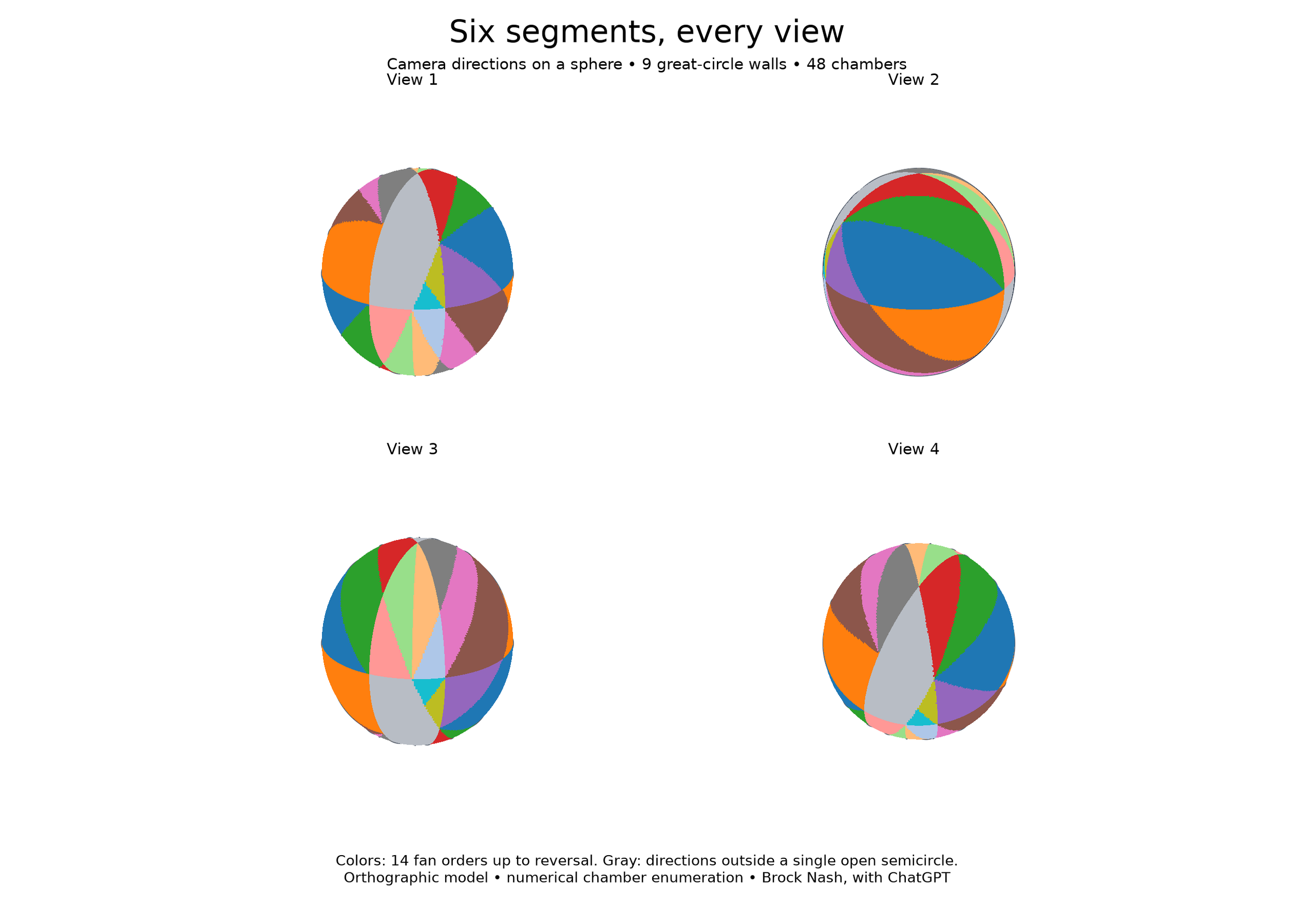
I explored the full space of camera directions with ChatGPT, treating each direction as a point on a unit sphere. For each pair, a critical direction satisfies k · (vᵢ × vⱼ) = 0: their projections become collinear. The 15 pairs reduce to nine distinct great-circle walls.
These walls divide the sphere into 48 chambers. Within each chamber, the signs of all pairwise comparisons remain unchanged.
Of these, 28 admit a linear fan order: all six projected directions fit within one open semicircle. Identifying each order with its reverse leaves 14 possibilities. The remaining 20 chambers fall outside that convention. Their rays still have a circular order, but no single open-semicircle fan.
The four views below show the same computed sphere from different angles. Colors identify the 14 fan orders up to reversal; gray marks the other chambers. Boundaries are sampled from the actual great-circle equations.
A hidden cube-symmetry arrangement
Why nine circles? Each pair of segments supplies a plane through the origin: k · (vᵢ × vⱼ) = 0. Intersecting that plane with the viewing sphere produces a perfect great circle. The 15 segment pairs collapse to nine distinct planes because the pairs 12/14/24, 15/16/56, and 34/36/46 each share a plane; the other six pairs give six separate planes.
There is a stronger structural explanation. Write a viewing direction as k = a v₂ + b v₃ + c v₅ = (a+b+2c, b+c, a+b). In these coordinates, the nine planes become a = 0, b = 0, c = 0, a = ±b, a = ±c, b = ±c. This is the standard B₃ reflection arrangement, associated with cube and octahedron symmetry. Choosing three coordinate signs and an ordering of their absolute values gives 2³ × 3! = 48 chambers. The coordinate change preserves the incidence structure, but changes angles and areas: our original triangles are a distorted version of the symmetric arrangement. Reference: reflection arrangements.
The network has 26 intersection points, 72 edges, and 48 triangular chambers. At 12 points two circles meet, at eight points three meet, and at six points four meet. Opposite viewpoints pair all these features. Its chamber-adjacency graph is also the edge graph of a polyhedron combinatorially equivalent to a truncated cuboctahedron: 48 vertices, 72 edges, and 26 faces.
This connects several descriptions of the same object: cube segments → comparison planes → spherical chambers → a transition graph of projected orders. A sign signature records which side of each plane the viewpoint occupies; crossing a boundary changes its associated comparisons. This is an example of the arrangement–oriented-matroid correspondence. Reference: matroids and oriented matroids.
Try other solids: what changes with viewpoint?
The same viewing-sphere idea can encode a different question: which faces of a convex solid can be seen? A face with outward normal n is front-facing when n · k > 0; its boundary n · k = 0 is another great circle. Regions now group viewpoints with the same visible face set. These are different maps from the six-segment ordering map above. A cube’s face-visibility map has only three distinct circles; adding the standard B₃ comparison planes subdivides it into 48 chambers.
One viewpoint, two connected views
Drag either canvas or use its arrow keys. Click a spot on the sphere to view the solid from that direction. Face colors and labels match the buttons; sphere colors identify entire visible-face combinations.
Select a face to highlight all directions from which it is front-facing. Select it again to clear.
Compare three graphs
These graphs share the viewpoint above. All edges are drawn, including faint dashed back edges. Click a sphere vertex to use that viewing direction; click a face node to highlight its visibility hemisphere; click a solid vertex to look from its direction. A sphere vertex is a boundary view, where some faces become edge-on.
Sphere intersection graph
Solid face-adjacency graph
Solid vertex-edge graph
Orthographic views of convex solids. Edge-on faces are boundary cases and do not count as visible. The standard B₃ grid stays fixed in world coordinates when you change the solid’s orientation; it illustrates a common coordinate partition, rather than claiming every solid has B₃ visibility symmetry.
Compare the counts
| Map | Great circles | Vertices | Edges | Zones |
|---|---|---|---|---|
| Cube face visibility | 3 | 6 | 12 | 8 |
| Square-pyramid face visibility | 5 | 12 | 28 | 18 |
| Tetrahedron face visibility | 4 | 12 | 24 | 14 |
| Octahedron face visibility | 4 | 12 | 24 | 14 |
| Standard B₃ arrangement | 9 | 26 | 72 | 48 |
Vertices and edges in this table belong to the spherical boundary network. Distinct zones were independently checked by feasibility enumeration of sign patterns. The square pyramid has four triple-circle intersection points and eight double-circle points; the tetrahedron and octahedron maps each have twelve double-circle points. Coincident boundaries are consolidated before counting.
From a 3-tuple to an m-tuple: a common mapping family
The cube offers a precise starting point. Away from boundaries, its six faces come in three opposite pairs, so exactly one face from each pair is visible. In cube-aligned coordinates, three coordinate signs give 2³ = 8 zones. The six face signs are not independent: the two signs in each opposite pair negate one another, so six face indicators encode only three independent choices. The sphere’s six intersection vertices lie along the six outward face normals. Joining them along boundary arcs gives an octahedral graph—the same graph obtained by joining cube faces that share an edge. Meanwhile, the eight spherical zones correspond to the eight cube vertices through cube-aligned coordinates v = (sign kₓ, sign kᵧ, sign k_z). This is a combinatorial correspondence; it does not identify every viewpoint in a zone with a different cube vertex.
The solid’s vertex-edge graph and face-adjacency graph are planar duals: a face becomes a node, and crossing a shared edge creates an adjacency. They need not have the same number of nodes. For the cube, the sphere intersection graph happens to match the face graph exactly. The other examples show why that equality is a special feature, rather than a universal rule. Reference: polytope face lattices and polarity.
For any convex polyhedron with m faces, place its outward normals in the rows of an m × 3 matrix A. Then define two maps:
gA(k) = Ak ∈ ℝᵐ
fA(k) = sign(Ak) ∈ {−1, 0, +1}ᵐ.
Each positive component identifies a visible face, each negative component a back-facing face, and each zero component an edge-on face. The live tuple readout above evaluates both functions for the current viewpoint. The same sign-map construction covers the original six-segment problem: use rows vᵢ × vⱼ instead of face normals, and the output records pairwise projected-orientation comparisons. Repeated proportional rows explain coincident great circles; the sign pattern alone does not automatically encode a single linear fan order.
There is a dimension-independent version: fA,b(x) = sign(Ax − b), with x an n-tuple, A an m × n matrix, and b an m-tuple. Setting b = 0 gives central hyperplane arrangements; on the unit sphere their boundaries are great hyperspheres. Thus one evaluation rule covers arbitrary dimensions and numbers of comparisons, with the geometry supplied by A and b. It is a universal evaluator within this family, rather than one fixed matrix that represents all shapes. Reference: hyperplane arrangements.
What can we recover?
The continuous map and its sign version retain different amounts of information. If A has full column rank, the full score tuple y = Ax determines x uniquely: x = (AᵀA)⁻¹Aᵀy. The sign tuple usually determines only a region. For example, the cube signature (+,+,+) in coordinate-sign notation means an entire octant, not one unique direction. Its inverse is naturally a set of solutions to inequalities, not a single viewpoint. We can choose a representative, but that choice adds a convention.
Even a one-to-one surface map is possible when we retain continuous information: k ↦ k / (|kₓ| + |kᵧ| + |k_z|) maps the unit sphere onto the surface of the octahedron |x|+|y|+|z|=1. Its inverse is radial normalization by Euclidean length. Each cube visibility zone lands on one octahedral triangular face, while the boundary network lands on its edges. This gives a concrete bridge between the spherical map and a polyhedral dual.
To recover graph relationships uniformly, we must also retain incidence data: which vertices belong to each edge and which edges belong to each face. Normals and signs describe viewing regions; incidence describes the solid’s connections. Together they provide a common representation from which these linked graphs can be built. Face visibility here uses convexity and orthographic projection. Nonconvex occlusion needs additional line-of-sight tests, so a sign-of-linear-functions model alone does not cover every possible shape or visibility question.
From a picture to a transition system
Crossing a wall changes the comparison signs. Connecting adjacent chambers gives a graph with 48 vertices and 72 edges. A camera path becomes a sequence of transitions, revealing both the final ordering and how we reached it.
That was the unexpected reward of following a small visual quirk: a drawing about square roots became an exploration of projection, permutations, and the geometry of viewpoint space.
Exploration and visualization by Brock Nash, developed with ChatGPT. These are computed plots rather than generative illustrations. Counts were checked by numerical linear-program feasibility enumeration for the six-vector orthographic model above; degenerate boundary views are excluded.
Generic formulas for circles, vertices, edges, and zones
All rows in the comparison table obey the same counting rules. Let g be the number of distinct great circles, after merging coincident circles, and let tr count the points where exactly r distinct circles meet. Count both antipodal points separately. For at least two distinct great circles:
Edges: E = Σr≥2 r tr
Zones: Z = 2 + Σr≥2 (r − 1)tr
An intersection of r circles has 2r incident edge ends. Counting both ends of each edge gives E = Σ r tr. Euler’s formula for the connected spherical network then gives V − E + Z = 2. Every pair of distinct great circles intersects twice, providing another check:
Σr≥2 [r(r − 1)/2] tr = 2[g(g − 1)/2] = g(g − 1).
| Map | Intersection signature | V | E | Z |
|---|---|---|---|---|
| Cube visibility | t₂ = 6 | 6 | 12 | 8 |
| Pyramid visibility | t₂ = 8, t₃ = 4 | 12 | 28 | 18 |
| Tetrahedron / octahedron visibility | t₂ = 12 | 12 | 24 | 14 |
| B₃ | t₂ = 12, t₃ = 8, t₄ = 6 | 26 | 72 | 48 |
When the circle count alone is enough
If no three circles meet at one point, all intersections are double intersections. The formulas simplify to:
V = g(g − 1), E = 2g(g − 1), Z = g² − g + 2.
The pyramid and B₃ arrangements have multi-circle intersections, so their circle counts alone do not determine the other columns. Their deviation from a generic arrangement is measured exactly by:
Z = g² − g + 2 − Σr≥3 [(r − 1)(r − 2)/2] tr.
Each triple intersection reduces the zone count by one relative to the generic count; each quadruple intersection reduces it by three. Nine generic great circles have 74 zones, whereas our B₃ arrangement has 74 − 8 × 1 − 6 × 3 = 48.
Where the circle count comes from
The geometry supplies g: count distinct normal directions, identifying all proportional nonzero normals, including opposites. For face visibility these are the face normals; for the original segment-order map they are the cross products vᵢ × vⱼ. Coincident circles must be merged before using the counting formulas. Circles that cross at a shared point remain distinct.
Thus (g; t₂, t₃, t₄, …) is a compact descriptor that determines every count in a table row. It is not a complete classification: different arrangements can share these numbers while having different detailed connectivity. The graph and incidence data preserve that additional structure. With only two circles, edges include distinct arcs joining the same two antipodal vertices; they must be counted separately.
